- STMicroelectronics Community
- Knowledge base
- MEMS and sensors
- How to use Machine Learning Core in automotive app...
- Subscribe to RSS Feed
- Mark as New
- Mark as Read
- Bookmark
- Subscribe
- Email to a Friend
- Printer Friendly Page
- Report Inappropriate Content
How to use Machine Learning Core in automotive applications using ASM330LHHX
- Subscribe to RSS Feed
- Mark as New
- Mark as Read
- Bookmark
- Subscribe
- Email to a Friend
- Printer Friendly Page
- Report Inappropriate Content
on 2022-07-26 05:03 AM
1. Software
The software tool that we use in this knowledge article is Unico-GUI, a graphical user interface (available for Linux, MacOS, and Windows) that supports a wide range of sensors and allows building an MLC program (even without any board connected = offline mode) and generating a sensor configuration file (UCF file).
2. Hardware
The STEVAL-MKI109V3 will be used in this tutorial to configure MEMS sensors and evaluate sensor outputs. Moreover, it has some advanced features for instance:
-
programmable voltage power supply
-
current consumption measurement
-
and communication protocol, which can be changed between SPI and I²C
The STEVAL-MKI109V3 can be used with different DIL24 adapter boards. In this tutorial we are going to use the STEVAL-MKI212V1, which is the DIL24 adapter board for ASM330LHHX, the IMU for automotive applications with the embedded machine learning core.
- ST resource page on MEMS sensor
- ST resource page on Explore Machine Learning Core in MEMS sensors
- Application note AN5296 on Machine Learning Core embedded in the ASM330LHXX
3. How to build the MLC configuration
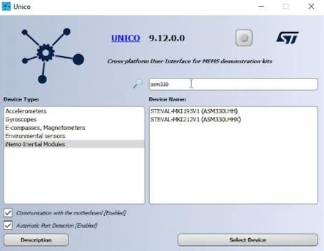
As a first step launch the Unico-GUI on the PC and select the adapter board STEVAL-MKI212V1, which contains the ASM330LHHX, the automotive IMU with the embedded machine learning core used in this knowledge article.
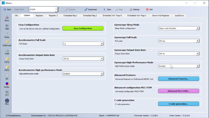
In the Unico-GUI main window, by clicking on the Option tab, it is possible to configure the main accelerometer and gyroscope settings. For this example, it has been selected:
-
AXL - 2g full scale and 104Hz output data rate
-
Gyroscope - 250dps full scale and 104Hz output data rate
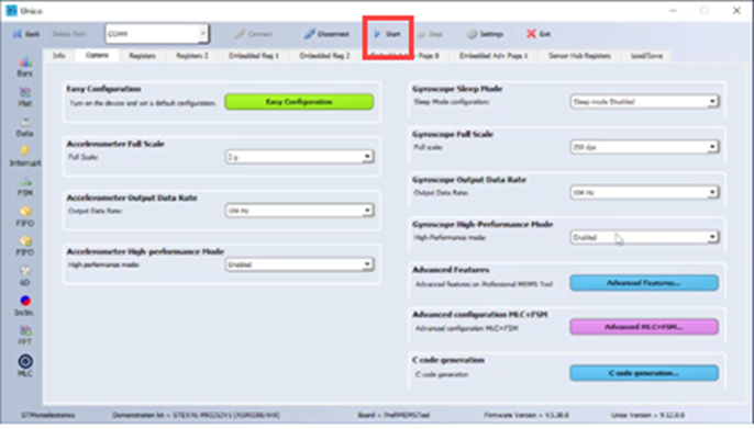
Clicking on the Start button on the top bar we are enabling the communication between the STEVAL-MKI109V3 and our PC.
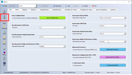
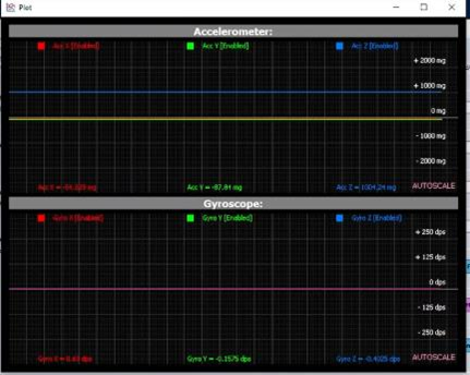
While clicking on the Plot tool we can visualize data coming from the sensor in real time.
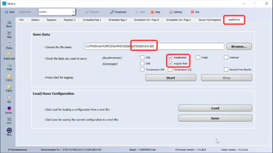
To start logging it is necessary to press on the "Load/Save tab", select the parameters to save, in this case it is necessary just the acceleration and the angular rate data, then it is needed to type the filename for the log, and acquire data for all the classes.
The classes that have been recorded and which will be detected with the ML algorithms for this knowledge article are:
-
Stationary
-
Moving
-
JackUp
-
Crash
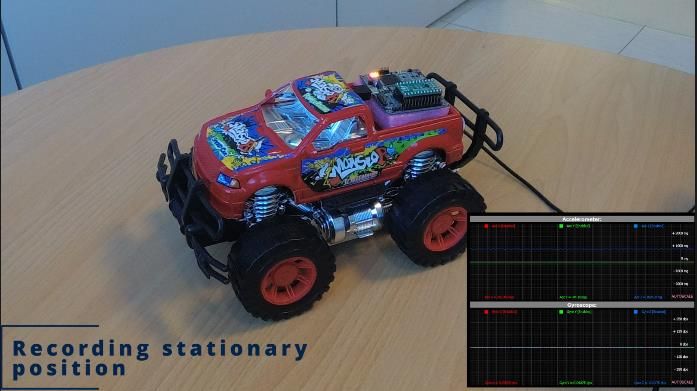
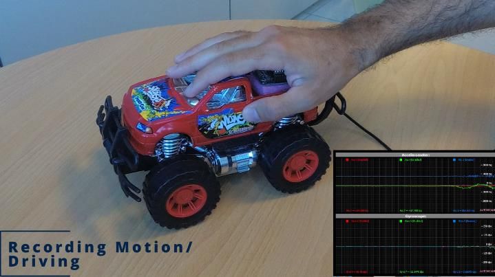
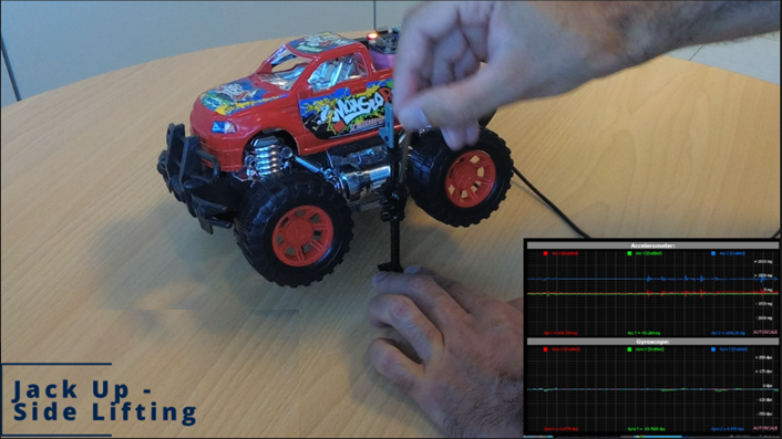
Once all the logs have been taken, it is recommended to analyze the logs for each class and to clean them. In this example Microsoft Excel was used.
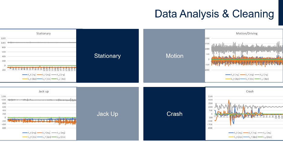
While analyzing the data logs, it was possible to notice that:
-
the main changes are in the accelerometer X and Y axes
-
the gyroscope does not provide additional information compared to the accelerometer
Therefore, it is possible to configure the MLC just using accelerometer data and select some features (like mean variance peak-to-peak) on accelerometer X and Y axes.
The next step is to import the data logs acquired in the MLC tool of Unico-GUI. In the "Data Patterns tab" of the MLC tool by clicking on the "Browse" button it is possible to select the corresponding data log files (multiple files can be selected simultaneously for the same class).
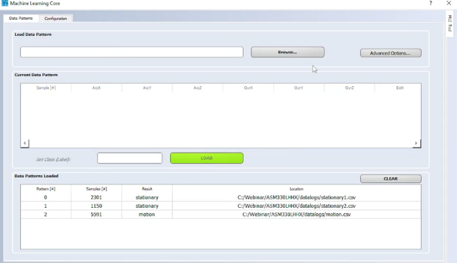
For all the data logs imported and for each class it is needed to assign a label, which is the class associated to that data.
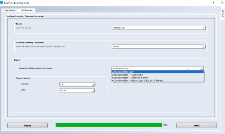
Once all the logs have been correctly imported, click on the “configuration” tab and proceed with the creation of the decision tree and the configuration file.
The configuration is for ASM330LHHX:
-
104 Hz data rate for Machine Learning Core (which is the same data rate used to acquire the data logs)
-
Accelerometer data only
-
2g full scale
-
104Hz data rate
-
-
No gyroscope is needed as when analyzing the data it was clear that it does not provide additional information for this application
Then it is needed to proceed with the configuration by selecting 1 decision tree and a window length of 104 samples. The window parameter specifies the number of samples the Machine Learning Core elaborates every time it has to identify a class. It can be from 1 to 255 and the latency of the MLC results will be related to this number. In this case with 104 Hz data rate, and 104 samples in the window get an equivalent time window of 1 second.
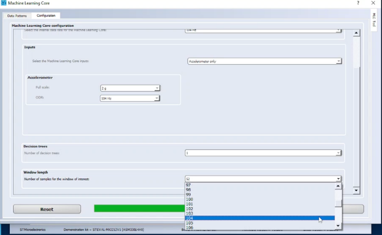
The filter configuration part is skipped for this example, that means that no filter is used on the input data.
In the features configuration section, it can be select which feature to use when building the decision tree.
Since from the data logs it was clear that there were some variations on the accelerometer X and Y axes, it is possible to select some features (like mean, variance, energy, peak2peak) on these axes, and also on the accelerometer norm.
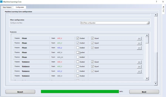
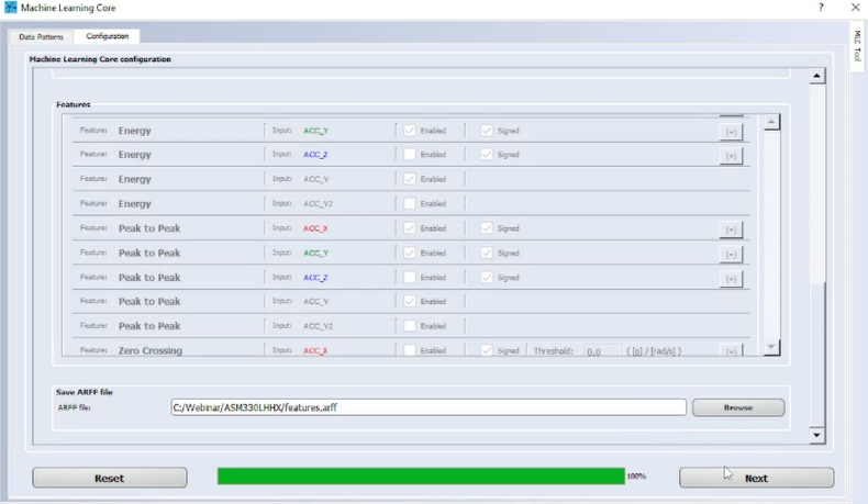
Now, the tool is generating the arff file, which is the file containing the features selected, computed in the 1 second window that was previously defined, using all the labeled data provided.
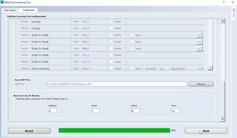
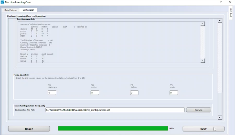
Then we need to decide which numeric values describe the different classes (These values are the outputs of the MLC and can be read in the MLC_SRC register of our device). We are using the values:
-
0 for stationary
-
4 for motion/driving
-
8 for jack up
-
12 for crash
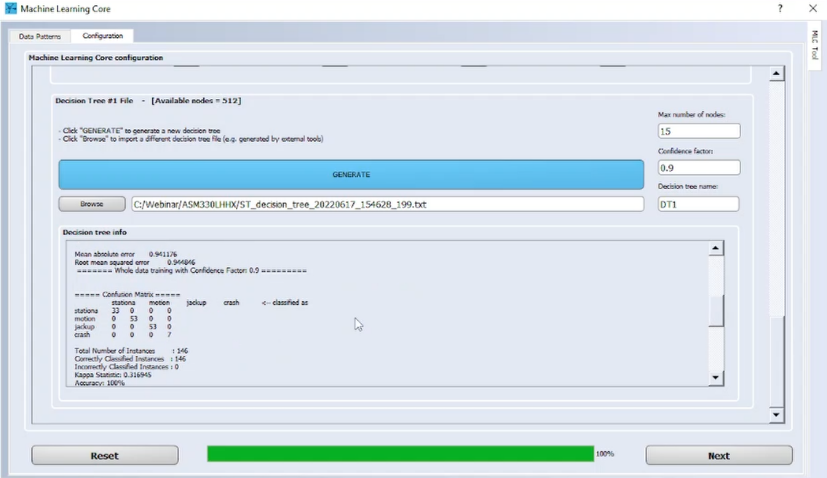
It is now possible to build following the configuration procedure, the decision tree, which uses some of the features previously defined by clicking on the Generate button, or alternatively it is possible to import decision trees generated by external tools. In the next section it is possible to select different filters, however for this example this part has been skipped. Finally, the tool can generate the UCF file with the Machine Learning Core configuration for ASM330LHHX , to embed the decision tree in the sensor configuration. Since the STEVAL-MKI109V3 with the ASM330LHHX DIL24 adapter (STEVAL-MKI212V1) is already connected to the PC, it allows to directly program the device, and evaluate this configuration.
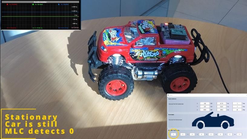
Finally, it is possible to check if the MLC works properly. The algorithm has to detect all the 4 recorded classes.
With the car still, we see the output 0, which means "Stationary".
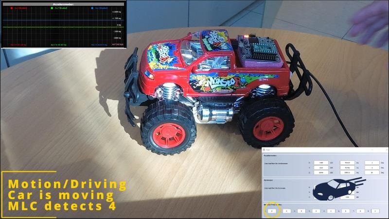
Moving the car forward and backward, the MLC output becomes 4.
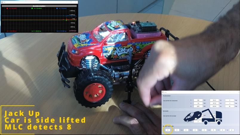
When the car is side lifted up, the MLC output becomes 8.
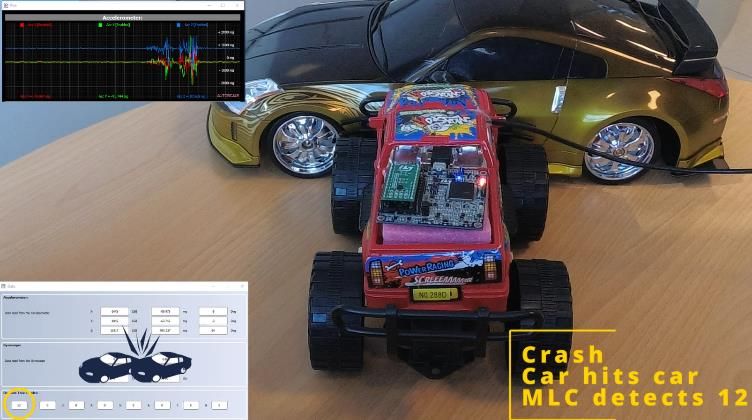
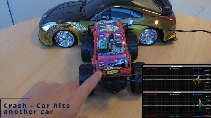
Finally, when the car hits another car, the MLC detects the class "crash", which has value 12.
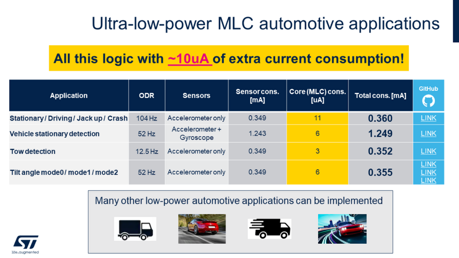
In this knowledge article it has been shown how to detect four different classes using the MLC in ASM330LHHX, but what is the current consumption? To have the MLC active, it is required just around 10 µA for this example. This is the additional current of the machine learning core, which has to be added to the sensor current consumption. Different configurations are possible - recognizing different classes - choosing a different data rate - or using different data (such accelerometer data only, or accelerometer + gyroscope). Here in the table you can see some examples that we have available in our GitHub repository for the same device.
